Show the code
pacman::p_load(ggstatsplot,plotly, crosstalk, DT, ggdist, zoo,gifski,ggiraph, gapminder, ggridges,gganimate,FunnelPlotR,knitr,tidyverse)Interactive Analytics on Resale Flat Prices, 2017 to 2023 Singapore
To uncover the salient patterns of the resale prices of 3-room, 4-room and 5-room public housing property by residential towns and estates in Singapore.
We will use appropriate analytically visualisation techniques as well as interactive techniques to enhance user and data discovery experiences.
The data can be downloaded here.
First load the r libraries.
pacman::p_load(ggstatsplot,plotly, crosstalk, DT, ggdist, zoo,gifski,ggiraph, gapminder, ggridges,gganimate,FunnelPlotR,knitr,tidyverse)Load the data set and filter using the flat type as we only focus on the resale price of 3-room, 4-room and 5-room.
prop_data <- read_csv("data/resale-flat-prices-based-on-registration-date-from-jan-2017-onwards.csv")
prop_data <- prop_data %>%
filter(flat_type == '3 ROOM' | flat_type == '4 ROOM' |flat_type =='5 ROOM')Let us first study the number of resale HDBs of different flat types from Jan 2017 to Feb 2023.
p1 <- prop_data %>%
  group_by(month) %>%
  ggplot(mapping = aes(x = prop_data$month)) +
  geom_bar_interactive(
    aes(tooltip = prop_data$month)
  )+
  theme_bw()+

  labs(title = "Monthly Sales Volume, from Jan 2017 to feb 2023", x = 'Time', y = 'Monthly Sales Volume',
       caption = "Singapore circuit breaker measures · 2020-04-07 to 2020-06-01 (1 month, 3 weeks, and 4 days)") +

  theme(axis.title.x=element_blank(),
        axis.text.x=element_blank(),
        axis.ticks.x=element_blank()) +
  geom_vline(aes(xintercept = '2020-04'),linetype = "dashed",color= 'red') +
  geom_vline(aes(xintercept = '2022-01'),linetype = "dashed",color= 'blue') +
  geom_vline(aes(xintercept = '2022-12'),linetype = "dashed",color= 'blue') +

  annotate("text",label = "Circuit Breaker", x = "2019-11",y=1000) +
  annotate("text",label = "2022", x = "2022-05",y=1000)+


  facet_wrap(~flat_type, nrow = 3)

girafe(
  ggobj = p1,
  width_svg = 6,
  height_svg = 6 * 0.618
)
Interactivity: By hovering the mouse pointer on the bar of interest, the respective month will be displayed.
Findings: During the 2 months of circuit breaker, the number of HDB resale flat transactions dropped 80% and recovered as soon as possible after the circular break ends. The volume of transactions resumed as soon as the circuit break ended.
Among the three flat types, the most popular type is the 4-room flats.
In 2022, the number of resale HDB peaks in September for all 3 types of HDB flats. In Feburary, the least number of HDBs been sold for all types. The reason might be due to the Spring Festival. Overall, the volume of transactions is quite stable compared with 2021.
prop_data_p2 <- prop_data %>%
  separate(month, into = c("year", "month"), sep = "-", convert = TRUE) %>%
  group_by(flat_type,year) %>%
  summarise(ave_price = round(median(resale_price),1),
            transation_volume = n(),
            mean_size = round(mean(floor_area_sqm),1))

tooltip_p2 <-
  c(paste( "Flat type:", prop_data_p2$flat_type,
           "\n Median resale price:" , prop_data_p2$ave_price,
           "\n Transaction volume:", prop_data_p2$transation_volume,
           "\n Mean size (sqm):", prop_data_p2$mean_size

))

p2 <-prop_data_p2 %>%
  ggplot(aes(x = year, y = ave_price,colour = flat_type))+
  geom_smooth(alpha = 0.1) +
  geom_point_interactive(aes(tooltip = tooltip_p2),size = 5) +
  theme_classic() +
  scale_x_continuous(breaks = seq(2017,2023,by = 1),limits = c(2017,2023)) +
  labs(title = "Resale Price of HDBs from 2017 to 2023", x = 'Year', y = 'Resale Price (SGD)')

girafe(
  ggobj = p2,
  width_svg = 12
)prop_data_p2 <- prop_data %>%
separate(month, into = c("year", "month"), sep = "-", convert = TRUE) %>%
filter(year == 2022) %>%
group_by(flat_type,month) %>%
summarise(ave_price = round(median(resale_price),1),
transation_volume = n(),
mean_size = round(mean(floor_area_sqm),1))
tooltip_p2 <-
c(paste( "Flat type:", prop_data_p2$flat_type,
"\n Median resale price:" , prop_data_p2$ave_price,
"\n Transaction volume:", prop_data_p2$transation_volume,
"\n Mean size (sqm):", prop_data_p2$mean_size
))
p2 <-prop_data_p2 %>%
ggplot(aes(x = month, y = ave_price,colour = flat_type))+
geom_smooth(alpha = 0.1) +
geom_point_interactive(aes(tooltip = tooltip_p2),size = 3) +
theme_classic() +
scale_x_continuous(breaks = seq(1,12,by = 1),limits = c(1,12)) +
labs(title = "Resale Price of HDBs in 2022", x = 'Month', y = 'Resale Price (SGD)')
girafe(
ggobj = p2,
width_svg = 12
)Interactivity: By hovering the mouse pointer on the data point(solid dot on the lines) of interest, the tooltip will be displayed. The tooltip includes the derived statistics of the median resale price, transaction volume and mean size.
Findings: The resale flat prices were relatively stable between 2017 and 2020. For 3-room HDB, the price decreased slightly from 2017 to 2019. Then the prices for all the 3 types began to rise from 2020. The difference of median transaction price between 3-room and 4-room is much larger than it between the 4-room and 5-room.
In 2022, the price of 5-room started to drop from October, while kept increasing of 3-room and 4-room.
Does the mean of the price per sqm differ among different flat types in 2022? First, let us explore the distribution of the mean price per sqm for different flat types.
prop_data_test1 <- prop_data %>%
  separate(month, into = c("year", "month"), sep = "-", convert = TRUE) %>%
  filter(year ==2022) %>%
  mutate(ave_price_per_sqm = round(resale_price/floor_area_sqm,1))

price_distribution <- prop_data_test1 %>%
  ggplot(aes(x = ave_price_per_sqm,y = flat_type)) +
  geom_density_ridges_gradient(color = 'white') +
  scale_fill_viridis_c(option = "C") +
  theme_ggstatsplot() +
  labs(title = "Distribution of Price",
       x = "Mean of Price psm (SGD)",
       y = "Flat Type")
price_distribution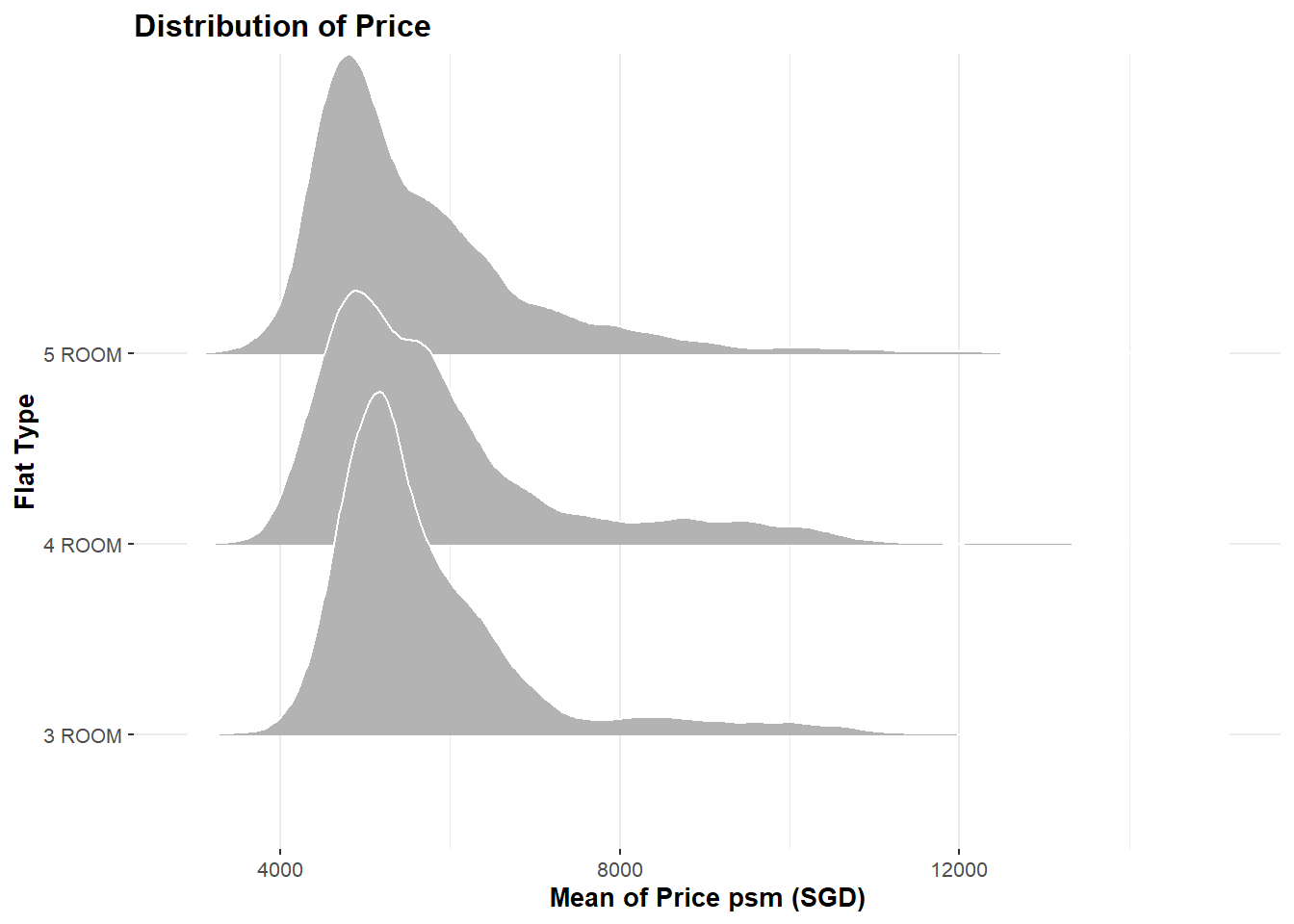
As the price per sqm of all three types skewed to left and does not follow a normal distribution, we use non-parametric anova test to compare the median of the price per sqm of 3 different flat types.
t1 <- ggbetweenstats(
  data = prop_data_test1,
  x = flat_type,
  y = ave_price_per_sqm,
  type = "np",
  mean.ci = TRUE,
  pairwise.comparisons = TRUE,
  pairwise.display = "s",
  p.adjust.method = "fdr",
  messages = FALSE
)

t1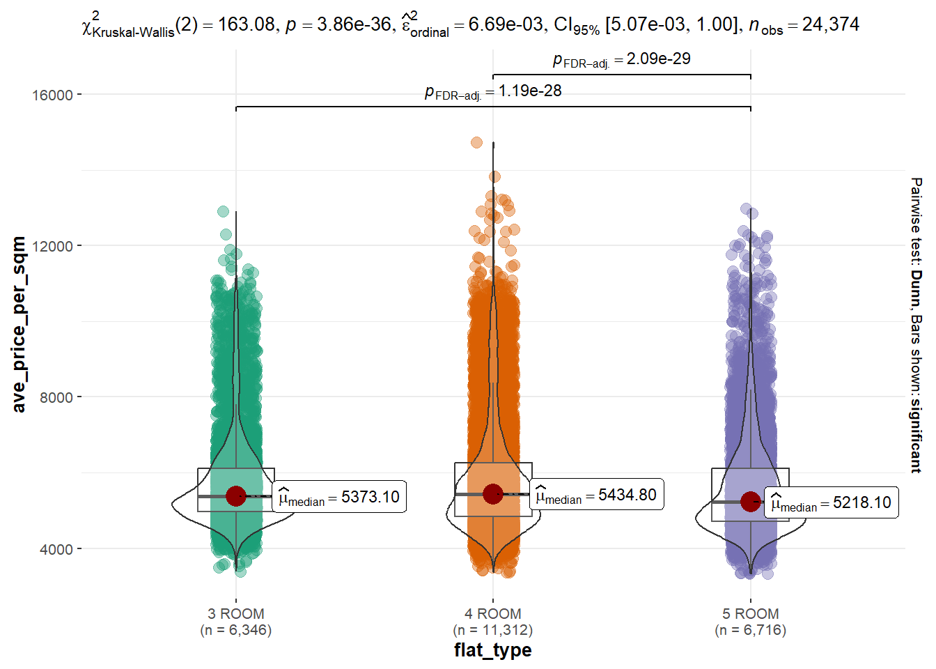
Kruskal-Wallis test is a non-parametric method for testing whether samples originate from the same distribution. Null hypothesis assumes that the groups are from identical populations. Alternative hypothesis assumes that at least one group comes from a different population than the others.
Conclusion: From the pairwise test result, we can conclude that: 1. There is no difference between the median price per sqm of 3-room and 4-room. 2. There are differences between the median price per sqm of 3-room and 5-room, and of 4-room and 5-room.
Plot the static ridgelines to show the distribution of average price/psm of flats in 2022 in Singapore for each residential towns.
 p3<- prop_data %>%
  separate(month, into = c("year", "month"), sep = "-", convert = TRUE) %>%
  filter(year ==2022) %>%
  group_by(town) %>%
  mutate(price_psm = resale_price/floor_area_sqm) %>%
  ggplot(mapping = aes(x=price_psm,
                       y = reorder(as.factor(town),-price_psm),
                       fill = after_stat(x)
                       )
         ) +
  geom_density_ridges_gradient( color = "white") +
  scale_fill_viridis_c(option = "C") +
  theme_bw() +

  theme(legend.position = "none") +
  theme(panel.grid = element_blank()) +
  labs(title = "HDB resale prices by residential towns, 2022 Singapore ",
       x = "Price psm (SGD)",
       y = "Planning Area")
p3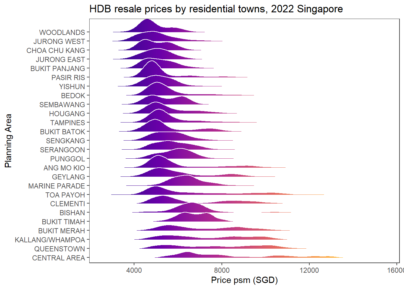
We can conclude that the resale of HDB in the areas such as woodlands, choa chu kang, jurong west are transacted at lower average price. And the price clustered around the average of $4000 to $5000 psm.
While the price of resale HDB in Bukit merah, queenstown and central area not only have a higher price, but also scattered from $6000 to $10000.
In general, HDBs in residential towns having lower price tend to have a lower variability.
Let us animate it.
ani1 <- prop_data %>%
  group_by(town) %>%
  mutate(price_psm = resale_price/floor_area_sqm) %>%
  mutate(date = as.Date(paste(month,"-01", sep=""))) %>%
  ggplot(mapping = aes(x=price_psm,
                       y = reorder(as.factor(town),-price_psm),
                       fill = after_stat(x)
                       )
         ) +
  geom_density_ridges_gradient( color = "white") +
  scale_fill_viridis_c(option = "C") +
  theme_bw() +

  theme(legend.position = "none") +
  theme(panel.grid = element_blank()) +
  labs(title = "HDB resale prices in {frame_time} Singapore",
       x = "Price psm (SGD)", y = "") +

  transition_time(date)
  anim_save('price_animation.gif',ani1)
From 2017 to 2020, the price is quite stable. Each curve stays at its original place. The shape of the curves with lower average price have much less change compares with those with higher average price.
However, from 2020 onwards, the curve starts to move to right. The average price almost increases by $1000 from 2020 to 2023.
Let us explore the remaining lease years of the HDB flats in different residential towns. The age of HDB flat = 99 years - remaining lease years.
prop_data_p4<- prop_data %>%
  mutate(age = 99-as.integer(substr(prop_data$remaining_lease,0,2))) %>%
  separate(month, into = c("year", "month"), sep = "-", convert = TRUE) %>%
  filter(year ==2022) %>%
  group_by(town)

tooltip <- function(y, ymax, accuracy = .01) {
  mean <- scales::number(y, accuracy = accuracy)
  sem <- scales::number(ymax - y, accuracy = accuracy)
  paste("Mean Age:", mean, "+/-", sem)
}

gg_point <- ggplot(data=prop_data_p4,
                   aes(x = reorder(town,age)),
) +
  stat_summary(aes(y = age,
                   tooltip = after_stat(
                     tooltip(y, ymax))),
    fun.data = "mean_se",
    geom = GeomInteractiveCol,
    fill = "lightblue"

  ) +
  stat_summary(aes(y = age),
    fun.data = mean_se,
    geom = "errorbar", width = 0.2, size = 0.2
  ) +
  facet_wrap(~flat_type)+
  coord_flip()+
  theme_bw() +

  theme(legend.position = "none") +
  theme(panel.grid = element_blank()) +
  labs(title = "Age of HDBs by residential towns, 2022 Singapore",
       y = "Age (years)",
       x = "Residential Town")
  #theme(axis.text.x = element_text(angle = 90, vjust = 0.5, hjust=1))

girafe(ggobj = gg_point,
       width_svg = 8,
       height_svg = 8*0.618)
Interactivity: By hovering the mouse pointer on the bar of interest, the respective mean age and standard error of mean will be displayed.
We can conclude that the HDB at punggol, sengkang are relatively new compared with the flats in marine parade and bukit timah. Moreover, 3-room flats are older than 4-room and 5-room flats.
prop_data_p5 <- prop_data %>%
  separate(month, into = c("year", "month"), sep = "-", convert = TRUE) %>%
  filter(year ==2022) %>%
  group_by(town,storey_range,flat_type) %>%
  summarise(median_price = median(resale_price))

tooltip_p5 <-
  c(paste( "Town:", prop_data_p5$town,
           "\n Storey:" , prop_data_p5$storey_range,
           "\n Median Price:",prop_data_p5$median_price
))

p5 <-  prop_data_p5 %>%
  ggplot(aes(x = reorder(town,median_price), y = storey_range, fill = median_price)) +
  geom_tile_interactive(tooltip = tooltip_p5) +
  scale_fill_gradient(low = "lightblue",high = "darkblue") +
  theme_bw() +
  labs(title = "Median Resale Price against Storey Range in Different Towns, 2022 Singapore",
       x = "Residential Town",
       y = "Storey Range") +
  theme(axis.text.x = element_text(angle = 90, vjust = 0.5, hjust=1)) +
  theme(axis.text.x = element_text(color = rep(c('black','orange','black','red','black','red'), time = c(16,2,4,2,1,1)))) +
  theme(axis.text.x = element_text(face = rep(c('plain','bold','plain','bold','plain','bold'), time = c(16,2,4,2,1,1))))
  #facet_wrap(~flat_type,nrow = 1)


girafe(
  ggobj = p5,
  width_svg = 10,
  height_svg = 10 * 0.618
)
Interactivity: By hovering the mouse pointer on the tile of interest, the tooltip will be displayed. The tooltip includes the town, story level and median resale price.
Findings: In general, the higher tiles tend to have darker blue. It means that the high floor HDBs are transacted at higher price. The tallest HDB flats are located in central area, queenstown and bukit merah. Recall what we have discovered about the distribution of price in different residential towns. The three towns have the highest median price in the past 5 years.
There are two towns, marine parade and bukit timah, where color are darker compared to others. It means that the HDB flats located are the same floor level are sold at higher price compared to other towns.
In general:
During circular break (2020 Apr to 2020 Jun), the volume of trasactions dropped 80% and resumed as soon as the circular break ends. The number of resale HDB flats transacted are slighter higher after circular break than it transacted before the circular break.
The price of resale HDBs were stable before 2020, and increased from 2020 to 2023.
The number of HDB flats sold was the highest in Sep 2022 and was the lowest in Feb 2022. The volume of transactions kept stable from 2021 to 2022.
For different flat types(3-room, 4-room, 5-room) :
The 4-rooms has the highest number of transaction.
The median price per sqm of 5 room is slightly lower than 3-room and 4-room.
The age of 3-room flats are the oldest.
For the flats in different residential town:
In Central Area, Queenstown and Bukit Merah: HDBs are the tallest and sold at the highest price.
In Centra Area, marine parade and Bukit Timah: HDBs are more expensive compared to others when they are at the same floor level.
In Punggol and Sengkang: many new HDBs are sold.